What is BEP on a pump curve?

BEP (Best Efficiency Point) is where the pump operates at maximum efficiency with minimum vibration and longest service life. It's the peak of the efficiency curve, typically 70-85% for well-designed pumps. API 610 recommends operating within 80-110% of BEP flow.

How do I find the operating point?

The operating point is where the pump curve and system curve intersect. Plot both curves on the same graph - the intersection shows the actual flow and head the pump will deliver in your system.

What do the affinity laws tell us?

Affinity laws relate flow (Q), head (H), and power (P) to speed (N) or impeller diameter (D): Q ∝ N (or D), H ∝ N² (or D²), P ∝ N³ (or D³). They're essential for predicting performance with VFD or impeller trim.

Why does my pump not deliver expected flow?

Actual operating point differs from design due to: higher system friction than calculated, partially closed valves, clogged strainers, impeller wear, or incorrect system head calculation. Compare actual vs design system curves.

Centrifugal Pump Curve Reading and Analysis - Complete Engineering Guide

1. Pump Curve Fundamentals

1.1 What a Pump Curve Shows

A complete centrifugal pump curve displays:

Curve	Description	Y-Axis	X-Axis
H-Q Curve	Head vs Flow (primary curve)	Head (m or ft)	Flow (m³/h or GPM)
Efficiency Curve	Pump efficiency vs Flow	Efficiency (%)	Flow
Power Curve	Shaft power vs Flow	Power (kW or HP)	Flow
NPSHr Curve	Required NPSH vs Flow	NPSHr (m or ft)	Flow

1.2 Curve Layout

Pump Characteristic Curve

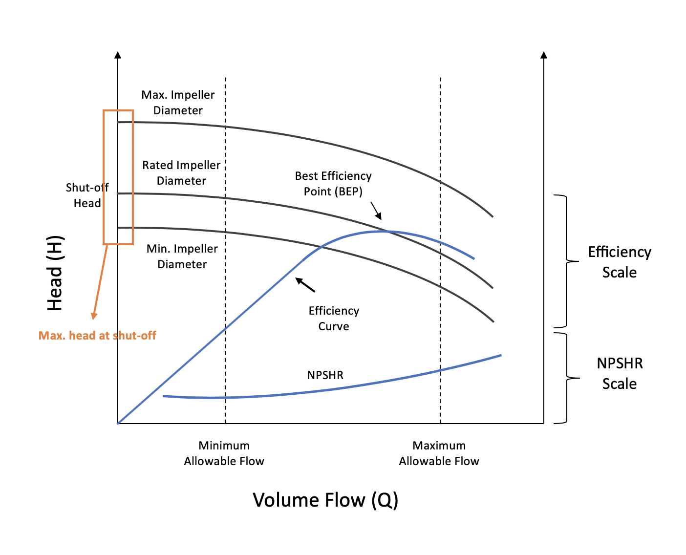
Pump characteristic curve showing H-Q curves for multiple impeller sizes. Each curve represents performance at different impeller diameters. Shut-off head (maximum head at zero flow) is shown at the left of each curve (Image credit: Shivansh231 - Wikimedia Commons, CC BY-SA 4.0)

Key Elements in Pump Curve:

Element	Description
H-Q Curves	Head vs Flow curve for each impeller diameter
Shutoff Head	Point where flow = 0 (leftmost point of curve)
Runout	Point of minimum head at maximum flow (rightmost)
BEP	Point of maximum efficiency

2. Head-Flow (H-Q) Curve

2.1 Key Points on H-Q Curve

Point	Definition	Location
Shutoff Head	Maximum head at zero flow	Left end of curve
Rated Point	Design flow and head	Specified duty point
BEP	Best Efficiency Point	Peak efficiency
Runout	Maximum flow at minimum head	Right end of curve

2.2 Curve Shape Characteristics

Curve Type	Head Rise to Shutoff	Stability	Application
Steep Rising	20-30%	Very stable	Parallel pumps, variable flow
Normal Rising	10-20%	Stable	General service
Flat	<10%	Marginal	Constant head required
Drooping	Drops before shutoff	Unstable	Avoid for parallel operation

Minimum Rise for Parallel Operation (API 610):

Rise to Shutoff = (H_shutoff - H_rated) / H_rated × 100%

Required: ≥ 10% rise for pumps operating in parallel

2.3 Reading Head and Flow

Step-by-step Process:

Locate required flow on X-axis
Draw vertical line to intersect pump curve
Read corresponding head on Y-axis
Verify curve (impeller diameter) being used

Example:

Required: 400 m³/h

From curve readings:
  - 280mm impeller: H = 85 m
  - 260mm impeller: H = 70 m
  - 240mm impeller: H = 55 m

If process requires 75 m head at 400 m³/h:
  → Select between 260mm and 280mm
  → Trim 280mm impeller to ~265mm

3. Best Efficiency Point (BEP)

3.1 BEP Definition

BEP is where:

Maximum hydraulic efficiency occurs
Minimum radial thrust on impeller
Minimum shaft deflection
Lowest vibration and noise
Longest bearing and seal life

3.2 Operating Regions (API 610)

Region	Flow Range	Characteristics	Recommendation
Preferred (POR)	80-110% of BEP	Optimal operation	Normal continuous operation
Allowable (AOR)	70-120% of BEP	Acceptable with monitoring	Short-term operation
Outside AOR	<70% or >120%	Risk of damage	Avoid

3.3 BEP Proximity Calculation

BEP Ratio = (Rated Flow / BEP Flow) × 100%

Example:
  Rated Flow = 450 m³/h
  BEP Flow (from curve) = 500 m³/h

  BEP Ratio = (450 / 500) × 100% = 90%

  Result: 90% of BEP → Within Preferred Operating Region ✓

3.4 Consequences of Operating Away from BEP

Condition	Consequences
Low Flow (<70% BEP)	Internal recirculation, temperature rise, suction recirculation, increased radial thrust, seal damage
High Flow (>120% BEP)	Cavitation risk, increased NPSHr, discharge recirculation, excessive vibration

4. Efficiency Curve

4.1 Efficiency Curve Shape

Efficiency │
    (%)    │              ●  BEP (82%)
    80     │           ╱    ╲
           │         ╱        ╲
    60     │       ╱            ╲
           │     ╱                ╲
    40     │   ╱                    ╲
           │ ╱                        ╲
    20     │╱                          ╲
           └──────────────────────────────
             0    200    400    600    800
                    Flow (m³/h)

4.2 Typical Efficiency Values

Pump Type	Typical BEP Efficiency
Small pumps (<20 kW)	50-70%
Medium pumps (20-200 kW)	70-80%
Large pumps (>200 kW)	80-90%
API 610 pumps	75-85% typical

4.3 Energy Cost of Efficiency Drop

Formula:

Annual Energy Cost = (Flow × Head × SG × 9.81 × Hours) / (3600 × η_pump × η_motor) × Rate

Where:
  Flow = m³/h
  Head = m
  SG = Specific Gravity
  Hours = Operating hours/year
  η = Efficiency (decimal)
  Rate = $/kWh

Example:

Flow = 500 m³/h, Head = 80 m, SG = 1.0
Hours = 8000 hr/yr, Rate = $0.10/kWh, η_motor = 0.95

At η_pump = 80%: Cost = $116,000/yr
At η_pump = 75%: Cost = $124,000/yr

5% efficiency drop = $8,000/year additional cost

5. Power Curve

5.1 Power Curve Characteristics

Power │
(kW)  │                           ╱ End of curve power
      │                         ╱
  80  │                       ╱
      │                     ╱
  60  │                   ╱
      │                 ╱
  40  │               ╱
      │             ╱
  20  │           ╱
      │  ●──────╱ Shutoff power
      └────────────────────────────
           Flow Rate →

5.2 Power Calculation

Shaft Power (kW) = (Q × H × ρ × g) / (η_pump × 3.6 × 10⁶)

Where:
  Q = Flow (m³/h)
  H = Head (m)
  ρ = Density (kg/m³)
  g = 9.81 m/s²
  η_pump = Pump efficiency (decimal)

5.3 Motor Sizing

Rule: Motor must handle power at end of curve (runout)

Motor Power ≥ (Power at runout) × Service Factor

Service Factor:
  - Standard service: 1.10
  - API 610: 1.15
  - Critical service: 1.25

6. NPSHr Curve

6.1 NPSHr Curve Behavior

NPSHr │
(m)   │                             ╱ Steep rise at high flow
      │                           ╱
  10  │                         ╱
      │                       ╱
   6  │                     ╱
      │                   ╱
   4  │               ╱
      │           ╱
   2  │  ●────╱ Relatively flat at low flow
      └────────────────────────────
           Flow Rate →

6.2 Key NPSHr Insights

Flow Range	NPSHr Behavior	Critical Check
Low flow	Relatively stable	Check at minimum continuous flow
BEP	Moderate increase	Check at rated point
High flow	Steep increase	Critical - check at runout

6.3 NPSH Margin Verification

NPSH Margin = NPSHa - NPSHr

API 610 Requirement:
  Margin ≥ MAX(1.0 m, 0.3 × NPSHr)

Example at 500 m³/h:
  NPSHa = 8.0 m (calculated)
  NPSHr = 5.0 m (from curve)
  Required margin = MAX(1.0, 0.3 × 5.0) = 1.5 m

  Actual margin = 8.0 - 5.0 = 3.0 m ✓

7. System Curve

7.1 System Curve Components

H_system = H_static + H_friction

Where:
  H_static = (Z₂ - Z₁) + (P₂ - P₁)/(ρg)  [Fixed]
  H_friction = K × Q²  [Varies with flow squared]

7.2 System Curve Plot

Head │
     │                        System Curve
     │                      ╱
     │                    ╱
     │                  ╱
     │                ╱  ← Friction head (varies with Q²)
     │              ╱
     │────────────╱
     │ ↑ Static head (constant)
     │
     └────────────────────────────
          Flow Rate →

7.3 System Curve Calculation Example

Given:
  Static head = 20 m
  Friction at 500 m³/h = 30 m

Calculate K:
  K = H_friction / Q² = 30 / 500² = 0.00012

System curve equation:
  H = 20 + 0.00012 × Q²

At different flows:
  Q = 0:     H = 20 m
  Q = 250:   H = 20 + 7.5 = 27.5 m
  Q = 500:   H = 20 + 30 = 50 m
  Q = 750:   H = 20 + 67.5 = 87.5 m

8. Operating Point Analysis

8.1 Finding Operating Point

The operating point is where pump curve intersects system curve:

Pump Curve and System Curve

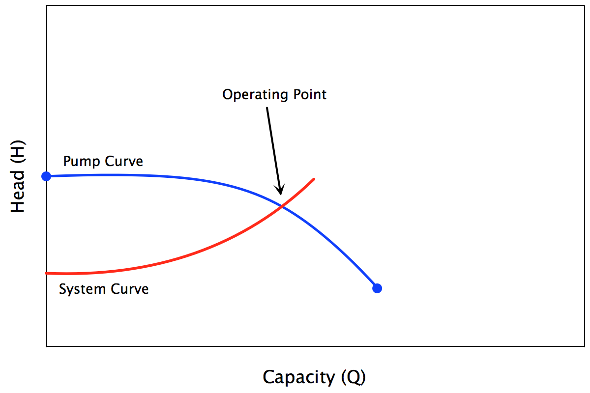
Intersection of Pump Curve and System Curve defines the Operating Point - this shows the actual flow and head at which the pump operates in that specific system (Image credit: Toomey usf - Wikimedia Commons, CC BY-SA 4.0)

8.2 Operating Point Scenarios

Scenario	Description	Solution
Pump curve below system	Pump cannot overcome head	Larger pump or reduce friction
Operating point far left of BEP	Over-sized pump	Trim impeller or use VFD
Operating point far right of BEP	Under-sized pump	Larger pump or reduce demand
No intersection	Wrong pump selection	Re-select pump

9. Affinity Laws

9.1 Speed Change (Constant Diameter)

Q₂/Q₁ = N₂/N₁
H₂/H₁ = (N₂/N₁)²
P₂/P₁ = (N₂/N₁)³

9.2 Diameter Change (Constant Speed)

Q₂/Q₁ = D₂/D₁
H₂/H₁ = (D₂/D₁)²
P₂/P₁ = (D₂/D₁)³

9.3 Worked Examples

Example 1: Speed Reduction

Original: N₁ = 2950 rpm, Q₁ = 500 m³/h, H₁ = 80 m, P₁ = 150 kW
New speed: N₂ = 2500 rpm

Ratio = 2500/2950 = 0.847

Q₂ = 500 × 0.847 = 424 m³/h
H₂ = 80 × 0.847² = 57 m
P₂ = 150 × 0.847³ = 91 kW

Power savings = 150 - 91 = 59 kW (39% reduction!)

Example 2: Impeller Trim

Original: D₁ = 280 mm, Q₁ = 500 m³/h, H₁ = 80 m
Required: H₂ = 70 m at same Q

D₂/D₁ = √(H₂/H₁) = √(70/80) = 0.935
D₂ = 280 × 0.935 = 262 mm

Trim impeller to 262 mm

9.4 Affinity Laws Limitations

Limitation	Impact
Efficiency changes	Laws assume constant efficiency; actual η varies slightly
Large changes	Accuracy decreases for >25% change
Viscous fluids	Additional correction needed
Specific speed	Different pump types respond differently

10. Parallel and Series Pump Operation

10.1 Parallel Operation

Principle: Add flows at same head

Parameter	Single Pump	Two Pumps (Parallel)
Head	H	H (unchanged)
Flow	Q	Q₁ + Q₂ ≈ 2Q
Curve shift	-	Horizontal (wider)

Formula:

Combined Head: H_combined = H_single (at any flow)
Combined Flow: Q_combined = Q₁ + Q₂ (at same head)

Example:

Single pump: 100 m³/h at 50 m head
Two pumps parallel: 200 m³/h at 50 m head

Requirements for Parallel Operation:

Rising head curve (no drooping)
Minimum 10% rise to shutoff
Similar pump characteristics
Check valves on each pump discharge

10.2 Series Operation

Principle: Add heads at same flow

Parameter	Single Pump	Two Pumps (Series)
Head	H	H₁ + H₂ ≈ 2H
Flow	Q	Q (unchanged)
Curve shift	-	Vertical (higher)